EXPLORE A SET OF MODELS
PHRAPL can generate and explore ‘all’ possible demographic scenarios or just a small set. Regardless of how many models are included in a PHRAPLanalysis, you need to be sure you know what and why a given set of models will be explored. Models can be as complicated as you want. But adding parameters to the models will significantly increase computational time.
Each model contains four matrices that specify colaescent events ($collapseMatrix), population sizes ($n0multiplierMap), population size changes ($growthMap), and scenarios of migration after each coalescent event ($migrationArray). Note that $migrationArray and migrationArray are not the same.
Explore a migrationArray object
Load a migrationArray object and explore model structure.
## This example explores a set of models for 3 population, where symmetric migration is forced and all possible topologies will be included.

setwd("/your_working_directory/")
library(phrapl)

#load a migrationArray object from github repository
load(url("https://github.com/ariadnamorales/phrapl-manual/raw/master/data/models_migrationArray/MigrationArray_3Pop_4K.allTopologies.symmMigration.rda"))
#load("MigrationArray_3Pop_4K.rda") 	## If file is stored in your working directory
Here we are interested in model 22. Therefore, type
# Explore model 22
migrationArray[[22]]
You will see something like this
> migrationArray[[22]]
$collapseMatrix
     [,1] [,2]
[1,]    1    2
[2,]    1   NA
[3,]    0    2

$complete
[1] TRUE

$n0multiplierMap
     [,1] [,2]
[1,]    1    1
[2,]    1   NA
[3,]    1    1

$growthMap
     [,1] [,2]
[1,]    0    0
[2,]    0   NA
[3,]    0    0

$migrationArray
, , 1

     [,1] [,2] [,3]
[1,]   NA    1    0
[2,]    1   NA    0
[3,]    0    0   NA

, , 2

     [,1] [,2] [,3]
[1,]   NA   NA    0
[2,]   NA   NA   NA
[3,]    0   NA   NA


attr(,"class")
[1] "migrationindividual"
For a quick visualization of this model, type
## Plot 3D model
PlotModel(migrationArray[[22]])
And voila
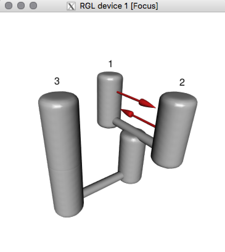
For more detailed explanation of how to plot model see section Plot models. For now let’s focus on understanding the structure of PHRAPLmodels (object class "migrationindividual").
$collapseMatrix
$collapseMatrix represents coalescent (or collapse) events between populations. **Columns represent colascent events and rows represent populations. Each coalescent event represents one parameter. **
In the previous example (for model 22), pop1 and pop2 coalesce at time one [,1]. Then, the ancestral population of these coaleses with pop3 at time two [,2]. This is a fully resolved topologoly. You would see somethinglike this:
> migrationArray[[22]]$collapseMatrix
     [,1] [,2]
[1,]    1    2
[2,]    1   NA
[3,]    0    2
Example for 3 populations where pop1 and pop2 coalesce at time one[,1], but pop3 does not coalesce with the ancestral population of pop1 and pop2. This is a isolation-with-migration model and the population that does not coalesce needs to be connected by migration to at least one of the other populations. You would see something like this:
> migrationArray[[20]]$collapseMatrix
     [,1] [,2]
[1,]    1    0
[2,]    1   NA
[3,]    0    0
Example for 3 populations where all three coalesce at time one [,1]. This is a polytomy. You would see something like this:
> migrationArray[[5]]$collapseMatrix
     [,1]
[1,]    1
[2,]    1
[3,]    1
Example for 3 populations where populations do not coalesce. This is an island model (migration-only model) and all populations need to be connected by migration to at least one population. You would see something like this:
> migrationArray[[1]]$collapseMatrix
     [,1]
[1,]    0
[2,]    0
[3,]    0
$n0multiplierMap
$n0multiplierMap represents population sizes after each coalesent vent. In the previous example (for model 22), all three populations have the same population size at all times.
> migrationArray[[22]]$n0multiplierMap
     [,1] [,2]
[1,]    1    1
[2,]    1   NA
[3,]    1    1
Example for 3 populations without collapse events where pop2 and pop3 have the same population size, and pop1 has a different population size at time 1. Values (1 and 2) do not indicate that one population is smaller or bigger than other(s), just that they are different parameters. You would see something like this:
> migrationArray[[xx]]$n0multiplierMap	## model not included in migrationArray from initial example.
     [,1]
[1,]    1
[2,]    2
[3,]    2
Example for 3 populations where pop2 and pop3 coalesce at time one and pop1 coalesces at time two. Before the first coalescetn event going backwards in time (e.g. in the present), pop2 and pop3 have the same population size, and pop1 has a different population size. After the first coalescent event, the ancestral population of pop2 and pop3, and pop1 are same size. You would see something like this:
> migrationArray[[xx]]$n0multiplierMap	## model not included in migrationArray from initial example.
     [,1] [,2]
[1,]    1    3
[2,]    2    3
[3,]    2   NA
$growthMap
$growthMap represents whether population sizes have changed (1=yes, 0=no). In the previous example (for model 22), the population size of the three populations remained constant.
> migrationArray[[22]]$growthMap
     [,1] [,2]
[1,]    0    0
[2,]    0   NA
[3,]    0    0
Example for 3 populations where pop2 and pop3 coalesce at time one and pop1 coalesces at time two. Population size of pop2 and pop3 does not change, but pop1does. Ancestral populations sizes do not change. You would see something like this:
> migrationArray[[xx]]$growthMap  ## model not included in migrationArray from initial example.
     [,1] [,2]
[1,]    1    0
[2,]    0   NA
[3,]    0    0
$migrationArray
$migrationArray represent migration events between populations before each coalescent event. Rows represent the 'source' population and columns represent 'destination' of migration.
In the previous example (for model 22), migration occurs between pop1 and pop2 only during the present (e.g. time one [,,,1]) and at the same rate. No migration between ancestral populations.
> migrationArray[[22]]$migrationArray
, , 1

     [,1] [,2] [,3]
[1,]   NA    1    0
[2,]    1   NA    0
[3,]    0    0   NA

, , 2

     [,1] [,2] [,3]
[1,]   NA   NA    0
[2,]   NA   NA   NA
[3,]    0   NA   NA
Example for 3 populations with assymmetric migration between pop1 and pop2 at the present (time one) and symmetric ancestral migration. Migration rates from pop2 to pop1 in the present, and between ancestral populations are the same. You would see something like this:
> migrationArray[[xx]]$migrationArray		## model not included in migrationArray from initial example.
, , 1

     [,1] [,2] [,3]
[1,]   NA    2    0
[2,]    1   NA    0
[3,]    0    0   NA

, , 2

     [,1] [,2] [,3]
[1,]   NA   NA    1
[2,]   NA   NA   NA
[3,]    1   NA   NA
Graphic summary
This figure summarizes what I have just described and represents an isolation with migration model where:
- PopA and popB coalesce at time one.
- PopA and popB have the same population size in the present and popC has a different size.
- Ancestral population sizes are the same among populations but different from the present.
- Population size of popC has changed (after the first coalescent event).
- Symmetric migration rates in the present and the past, but at different rates.
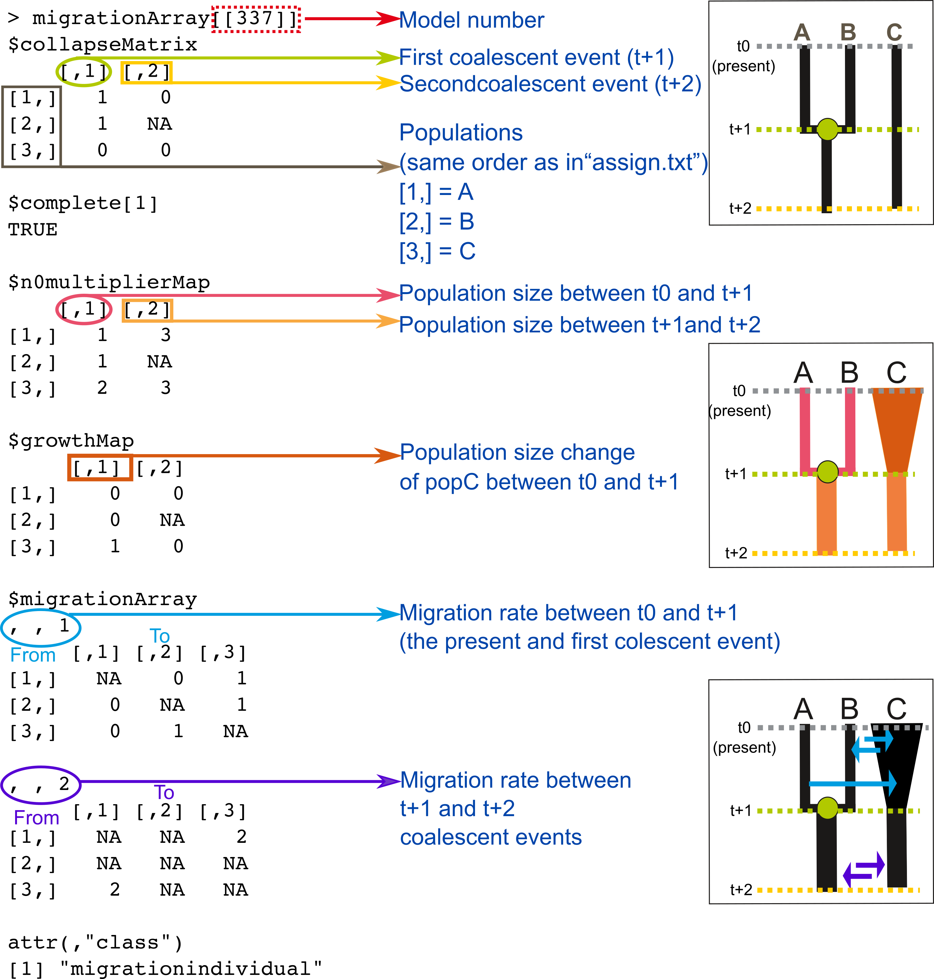
Fig. Structure of PHRAPL models.