Tutorial 2: Sensitivity analyses and fixing migration time
This tutorial assumes that you have already followed and understand the steps of Tutorial 1
The first part of this tutorial will walk you through a PHRAPL analysis to recalculate model weights (wAIC) in gradually increasing subsets of loci and how to handle haploid and diploid loci in the same analysis. The figure below represents how results from these type of analyses could be summarized. Each column represents one model, each row represent a subset of loci (gradually increasing in number), and the color represents the model weight (wAIC analogous to model probability), that is higher as it gets darker.
Then, the second part, will show you how to compare models of no gene flow, gene flow only during early stages of divergence, constant gene flow throughout time, or secondary contact (as represented in the figure below, from left to right). To test such scenarios with different time intervals of gene flow, we use a model with a fixed topology and a fixed migration matrix (direction of gene flow between species or populations) that may be symmetric (red arrows in the figure) and/or asymmetric (green arrows in the figure). We assume that such a model was already inferred as the ‘best’ model from a bigger set in a previous analysis. We only change when gene flow starts or stops.

This is what we did in our “Speciation with Gene Flow in North American Myotis Bats” paper. But for this tutorial, we use smaller datasets. For the first part, we use an example dataset of 5 loci from 2 populations Plethodon salamanders. In the second part, we analyze a bigger dataset of 1200 loci from 2 unisexual and sexual species of Ambystoma salamanders. We have highlighted with orange asterisks those blocks of code that constitute the minimum steps that must be followed. Run all the commands in your shell terminal (not in your R terminal). You can run Part 2 without having to run Part 1.
- Part 1: Recalculate model weights (wAIC) in subsets.
- Part 2: Constant vs ancestral vs recent gene flow
Part 1: Recalculate model weights (wAIC) in subsets.
Activate conda environment and load R
*****************************************************************## activate conda environment and load R
conda activate OX_env_phrapl
R
Download files and scripts – run them in the background
The following commands will download all the required files and scripts for this tutorial. And, the analysis will start running in the background while we discuss what is happening in each step. In your terminal type:
**************************************************************************download.file("https://raw.githubusercontent.com/ariadnamorales/phrapl-manual/master/data/exampleData/1.Subsampling_GridSearch_Post.R", destfile="1.Subsampling_GridSearch_Post.R")
system("R CMD BATCH 1.Subsampling_GridSearch_Post.R > 1.Subsampling_GridSearch_Post.R.out")
Discuss how to set up a PHRAPL analysis
Do not run the following commands in your terminal. This analysis is already running in the background. Here we are discussing what is going on and how you can change settings for future analyses.
Load input files from GitHub
Housekeeping commands to load libraries, input files, a precomputed model set (a.k.a. migrationArray), and create output directories.
setwd("/working_path/sensitivityAnalyses")  # <----- Change this line if your are running the tutorial step by step

## Create output dirs
	system(paste0("mkdir ", getwd(),  "/results"))
	system(paste0("mkdir ", getwd(),  "/results/RoutFiles"))

## Load libraries and functions
library(ape)
library(partitions)
library(phrapl)

## migrationArray
load(url("https://github.com/ariadnamorales/phrapl-manual/raw/master/data/sensitivityAnalyses/example/input/MigrationArray_2pop_3K.rda"))

## Input Files
currentAssign<-read.table(file="https://raw.githubusercontent.com/ariadnamorales/phrapl-manual/master/data/sensitivityAnalyses/example_with_outputFiles/input/Pleth_align.txt", head=TRUE)
currentTrees<-ape::read.tree("https://raw.githubusercontent.com/ariadnamorales/phrapl-manual/master/data/sensitivityAnalyses/example_with_outputFiles/input/Pleth_bestTree.tre")
Subsampling
If you followed tutorial 1, you already know what is happening in Subsampling and GridSearch.
########################
### 1. Subsampling  ####
########################

## Define arguments
subsamplesPerGene<-10
nloci<-5						## IMPORTANT: one of these loci is haploid
popAssignments<-list(c(3,3))


## Do subsampling
observedTrees<-PrepSubsampling(assignmentsGlobal=currentAssign,observedTrees=currentTrees,
popAssignments=popAssignments,subsamplesPerGene=subsamplesPerGene,outgroup=FALSE,outgroupPrune=FALSE)

### You will see this error message:
### Warning messages:
#		1: In PrepSubsampling(assignmentsGlobal = currentAssign, observedTrees = currentTrees,  :
#	  Warning: Tree number  1 contains tip names not included in the inputted assignment file. These tips will not be subsampled.
### This is because we exclude a few individuals from the Assignment File to reduce computational time for the sake of this tutorial.

## Get subsample weights for phrapl
subsampleWeights.df<-GetPermutationWeightsAcrossSubsamples(popAssignments=popAssignments,observedTrees=observedTrees)

## Save subsampled Trees and weights
save(list=c("observedTrees","subsampleWeights.df"),file=paste0(getwd(),"/phraplInput_Pleth.rda"))
GridSearch
Here, look at the GridSearch arguments popScaling and print.ms.string. With popScaling you can specify if any (or all) of your loci is haploid (0.25 Ne) or diploid (1 Ne). The order of these values should match the order of the trees in your input file. In this example, a tree from mitochondrial locus is listed first. Setting print.ms.string=TRUE will allow you to use the output file to recalculate wAIC is subsets of loci, that file is named 1.Subsampling_GridSearch_Post.Rout in this tutorial.
######################
### 2. GridSearch  ###
######################

## Search details
modelRange<-c(1:5)
popAssignments<-list(c(3,3))  					## number of indvs per pop that will be subsampled
nTrees<-100
subsamplesPerGene<-10
totalPopVector<-list(c(4,4))     				## total number of indvs per pop
popScaling<-c(0.25, 1, 1, 1, 1)					## IMPORTANT: one of these loci is haploid --> 1/4 Ne

## Run search and keep track of the time
startTime<-as.numeric(Sys.time())

result<-GridSearch(modelRange=modelRange,
	migrationArray=migrationArray,
	popAssignments=popAssignments,
	nTrees=nTrees,
	observedTree=observedTrees,
	subsampleWeights.df=subsampleWeights.df,
	print.ms.string=TRUE,						## IMPORTANT: setting this argumemnt as TRUE will allow you to
												##				recalculate wAIC in subsets of loci
	print.results=TRUE,
	debug=TRUE,return.all=TRUE,
	collapseStarts=c(0.30,0.58,1.11,2.12,4.07),
	migrationStarts=c(0.10,0.22,0.46,1.00,2.15),
	subsamplesPerGene=subsamplesPerGene,
	totalPopVector=totalPopVector,
	popScaling=popScaling,
	print.matches=TRUE)

# Grid list for Rout file
gridList<-result[[1]]

#Save the workspace and cleaning
save(list=ls(), file=paste0(getwd(),"/results/Pleth_",min(modelRange),"_",max(modelRange),".rda"))
system(paste0("mv ", getwd(), "/1.Subsampling_GridSearch_Post.Rout ", getwd(), "/results/RoutFiles/1.Subsampling_GridSearch_Post.Rout"))
system(paste0("rm ", getwd(), "/1.Subsampling_GridSearch_Post.R.out"))
When you see these output files go to next step: 
Post-process
We will start running commands in our terminals here:
Here we make sure that the analysis ran correctly, calculate model averages (including all loci), and plot the ‘best’ model.
*****************************************************************#setwd("/working_path/sensitivityAnalyses") ### working Dir in previous script (if you changed it.)
########################
### 3. Post-process ###
########################
## load libraries and custom functions
library(phrapl)
## migrationArray
load(url("https://github.com/ariadnamorales/phrapl-manual/raw/master/data/sensitivityAnalyses/example/input/MigrationArray_2pop_3K.rda"))
## If different models (from the same migrationArray file) were run separatly, the output can be concatenated.
totalData<-ConcatenateResults(rdaFilesPath=paste(getwd(),"/results/",sep=""),rdaFiles=NULL,addAICweights=TRUE,addTime.elapsed=FALSE)
modelAverages<-CalculateModelAverages(totalData, parmStartCol=9)
## Save output to a txt file
write.table(totalData, file=paste(getwd(),"/results/totalData.txt",sep=""), sep="\t", row.names=FALSE, quote=FALSE)
## Plot the best model
PlotModel(migrationArray[[3]], taxonNames=c("S","N"))
#PlotModel(migrationArray[[5]], taxonNames=c("S","N"))
#PlotModel(migrationArray[[4]], taxonNames=c("S","N"))
Plot of the ‘best’ model: 
Sensitivity analyses: generate subsets.
Each run will generate two files, one with extension rda and one with extension Rout. The rda files are used to post-process the results and calculate final model averages (as done above). The Rout files will contain information of the GridSearch performance, we are interested in the match vector, which contains information of the number of times that each subsample in each locus was found in the simulated distribution of trees.
This figure represents a GridSearch output listing parameter grids, grid values (or grid points), running settings (such as nsam, nreps, opts), results (AIC and lnL), and the number of matches. There will be one list per model and per grid parameter combination.
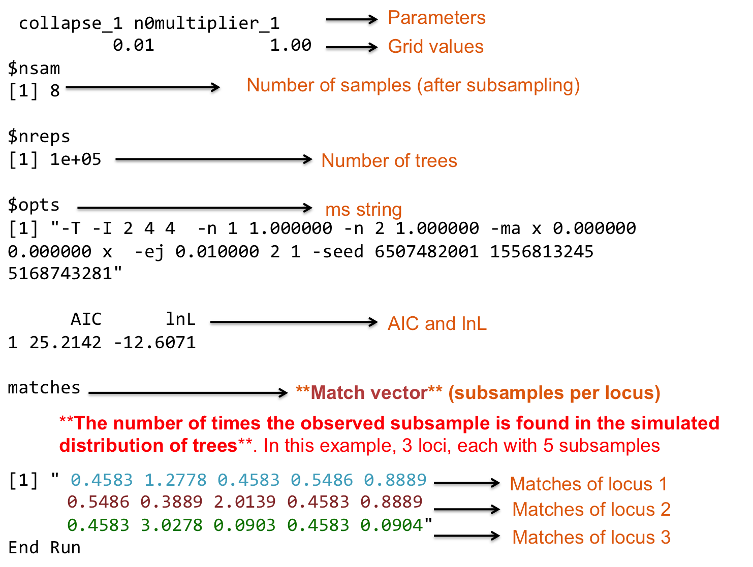
Before recalculating model averages per locus (or subset of loci), it is necessary to extract the match vectors. Then, the function GenerateSetLoci will re-calculate AICs and parameter estimates for subsets of loci. This can either be done for independent subsets of loci (cumulative=FALSE) or for cumulative subsets (cumulative=TRUE, in which the second subset is added to the first subset, and then the third subset is added to these, etc). lociRange gives the number of loci in the original analysis and NintervalLoci gives the desired number of loci in each subset, which must be a multiple of the total number of loci. If the models in the original analysis are only a subset of models in the migrationArray, this modelRange must be specified as well. The output of GenerateSetLoci is an rda file for each locus subset (numbered in order with a numerical suffix, i.e., _1, _2, _3, etc). Note that subsets are taken in order from the original output files. Note: We are using a GenerateSetLoci version downloaded with this tutorial’s files (not the one included in the phrapllibrary). A few changes were made to make the process easier to follow. You can use it for further analyses, make sure to load it as a source file.
################################
### 4. Sensitivity analyses  ###
################################

## Load libraries
library(gplots)
source("https://github.com/ariadnamorales/phrapl-manual/raw/master/data/sensitivityAnalyses/example/scripts/GenerateSetLoci_cum8_v3.R")

## Load phrapl input (subsampled dataset)
load(paste0(getwd(),"/phraplInput_Pleth.rda"))

## Create output folders
system(paste("mkdir ", getwd(), "/results/subsets",sep=""), ignore.stderr=TRUE)

#########################################################
### Define arguments (some of these were already defined whe running GridSearch)
nloci<-5
NintervalLoci<-1				## new parameter --> required by GenerateSetLoci
modelRange<-c(1:5)
lociRange<-c(1:5)				## new parameter --> required by GenerateSetLoci
subsamplesPerGene<-10
popAssignments<-list(c(3,3))
collapseStarts<-c(0.3, 0.58, 1.11, 2.12, 4.07)
migrationStarts<-c(0.1, 0.22, 0.46, 1, 2.15)
n0multiplierStarts<-NULL
setCollapseZero<-NULL
nTrees<-100
dAIC.cutoff<-2
nEq<-100
subsampleWeightsVec=subsampleWeights.df[[1]][,1]
migrationArrayShort<-migrationArray[modelRange]

#####################################
### Load files with match vectors ###
rdaFilename<-paste(getwd(),'/results/Pleth_1_5.rda', sep="")

system(paste("grep matches -A1 ",getwd(),"/results/RoutFiles/1.Subsampling_GridSearch_Post.Rout | grep -v matches | grep 0 > ",getwd(),"/results/RoutFiles/matches_2.RunGridSearch.Rout.txt", sep=""))
RoutFilename<-read.table(file=paste(getwd(),'/results/RoutFiles/matches_2.RunGridSearch.Rout.txt', sep="") ,skip=1)

#####################################################
### Recalculate model averages in subsets of loci ###

# Command line to run function GenerateSetLoci
GenerateSetLoci(lociRange=lociRange,NintervalLoci=NintervalLoci,RoutFilename,rdaFilename,migrationArray=migrationArray,modelRange=modelRange,subsamplesPerGene=subsamplesPerGene,collapseStarts=collapseStarts,migrationStarts=migrationStarts,n0multiplierStarts=n0multiplierStarts,setCollapseZero=setCollapseZero,cumulative=TRUE,nTrees=nTrees,dAIC.cutoff=2,nEq=nEq, subsampleWeightsVec=subsampleWeightsVec)
When you see these output files go to next step: 
Postprocess RDA files per subset
Here we re-calculate model averages (for each subset of loci).
*****************************************************************#########################################
### Postprocess RDA files per subset ###
# Set paths to input and output files ---> Files created by GenerateSetLoci.
pathSubsets<-paste0(getwd(), "/results/subsets/")
pathtotalData_subsets<-paste0(getwd(), "/results/subsets/")
# Loop to analyze output files ----> Will generate a totalData file per subset per model
# You may need to create one folder per subset and move files to each folder
for(i in 1:5){ ## ------> Be careful to specify the total number of subsets (in this case 5)
totalData<-list()
totalData<-ConcatenateResults(rdaFilesPath=paste0(getwd(), "/results/subsets/subset",i,"/"),rdaFiles=NULL, migrationArray, rm.n0=TRUE, longNames = TRUE, outFile=NULL,addAICweights=TRUE,addTime.elapsed=FALSE, nonparmCols = 4)
write.table(totalData, file=paste(pathtotalData_subsets,"totalData_subset",i,".txt",sep=""), sep="\t", row.names=FALSE)
}
When you see these output files go to next step: 
Plot subsets
Here we plot the wAIC values of each model and subset. If the wAIC of the top models is very similar when the entire dataset is analyzed, that may indicate that more data could add information to distinguish between models. Seeing how the wAICs change as we add data can help us to decide when/if we have enough data, if a single model achieves the highest support far away from the rest.
*****************************************************************########################
### 5. Plot subsets ###
########################
pathInputFiles<-paste0(getwd(), "/results/subsets/")
totalData_list<-list.files(pathInputFiles, pattern="*.txt", full.names=FALSE)
totalData_files<-c()
for(x in 1:length(totalData_list)){
totalData_files<-append(totalData_files,list(read.table(paste(pathInputFiles,totalData_list[x],sep=""),header=TRUE, fill=TRUE, sep="\t")))
}
#Sort each dataframe by model
totalData_filesSorted<-c()
for(x in 1:length(totalData_list)){
totalData_filesSorted<-append(totalData_filesSorted,list(totalData_files[[x]][order(totalData_files[[x]]$models),]))
}
#Create a dataframe with all models and their wAIC
model_wAIC<-data.frame("models"=c(1:5),row.names=NULL)
for(x in 1:length(totalData_list)){
model_wAIC[,paste("Subset ",x,sep="")]<-totalData_filesSorted[[x]][,"wAIC"]
}
########################
## Define plot settings
## Row Labels
row.label<-c()
setLoci<-0
for(i in 1:length(totalData_list)){
setLoci<-setLoci+8 ##loci interval
row.label<-append(row.label, c(paste(setLoci, " Loci",sep="")))
}
## Row labels --->
row.labels <- rep("", 5)
## Col Labels
col.label<-seq(1:5)
## Color scale
bks<-c(seq(0,0.99,by=0.05))
lm.palette <- colorRampPalette(c("light yellow","orange", "tomato"), space = "rgb")
## Possition of the plot and legend
lmat <- rbind(c(0,3,3,3),c(2,1,1,1),c(0,0,0,4))
lwid <- c(0.2,1,1,1)
lhei <- c(0.3,2.1,0.5)
pdf(file=paste(getwd(),"/results/wAICinSubsets.pdf", sep=""), width=9, height=7)
heatmap.2(as.matrix(t(model_wAIC[2:length(model_wAIC)])), lmat = lmat, lhei=lhei,lwid=lwid,
Rowv=FALSE,Colv=FALSE, dendrogram="none", trace="none",
margins=c(2,12),
col=lm.palette(length(bks)-1), breaks=bks,
#colsep=1:5,
rowsep=1:(length(model_wAIC)-1), sepcolor="white",
#labRow=row.labels,
#labCol=col.label,
key = TRUE,
#keysize =1.0,
density.info=c("density"),
denscol=tracecol,
key.xlab="wAIC",
key.par=list(mar=c(4,4,4,4)),
main="wAIC for each model per locus")
dev.off()
This is the plot you should recover if all the steps of this tutorial were succesful. However, these results are not informative. We could not draw any conclusions because we did not include enough or more informative data. 
With many more loci and models, you could build a plot such as this one.

Part 2: Constant vs ancestral vs recent gene flow
You can run Part 2 without having to run Part 1. For this section make sure that you understand how `PHRAPL` models are structured in an R object. You need to be familiar with what is a migrationArray object and its components: $collapseMatrix, $n0multiplierMap, $growthMap, $migrationArray. See this explanation if you need a reminder.
- Note: the object
migrationArray, is alistobject that is the model, actually you can call it however you want. It includes anarraycalled$migrationArraythat includes the migration matrices within such model/object. This may be confusing but for historical reasons that is how it was developed…
** Only run the blocks of code highlighted with orange asterisks. Run the commands in your shell terminal (not in your R terminal).**
Activate conda environment and load R
*****************************************************************## activate conda environment and load R
conda activate OX_env_phrapl
Download files and scripts – run them in the background
The following commands will download all the required files and scripts for this tutorial. And, the analysis will start running in the background while we discuss what is happening in each step. In your terminal type:
*****************************************************************wget https://github.com/ariadnamorales/phrapl-manual/raw/master/data/tutorial2.2/scripts/2.2.buildModels_loadData_Subsampling_GridSearch_Post.R
R CMD BATCH 2.2.buildModels_loadData_Subsampling_GridSearch_Post.R > 2.2.buildModels_loadData_Subsampling_GridSearch_Post.Rout
How to generate models with different time intervals of gene flow
To generate such models, we need to start with “traditional” PHRAPL models with and without gene flow.
In this tutorial we, start with 2 models.
## load R (if you haven´t)
## Load libraries
library(phrapl)

## get migrationArray with 2 models (no gene flow and asymmetric gene flow)
load(url("https://github.com/ariadnamorales/phrapl-manual/raw/master/data/tutorial2.2/models/MigrationArray_2Pops_2models_noMig_assymMig.rda"))

length(migrationArray)
#[1] 2
No gene flow
The first model includes 2 sister populations/species with a single coalescent event, same population size, no changes in population size, and no gene flow.
migrationArray[[1]]
Returns this output:
$collapseMatrix
     [,1]			## For these 2 groups/populations/species
[1,]    1			## there is only one coalescent event (seeing from the present to the past)
[2,]    1			## or single divergence event (fseeing rom the past to the present).

$complete
[1] TRUE

$n0multiplierMap
     [,1]
[1,]    1				## Same population size in group/population/species 1  --> "1"
[2,]    1				## Same population size in group/population/species 2  --> "1"

$growthMap
     [,1]
[1,]    0				## No changes in population size in group/population/species 1  --> "0"
[2,]    0				## No changes in population size in group/population/species 2  --> "0"

$migrationArray
, , 1					## There is only one ", , 1" interval assigned to gene flow
						## therefore, it is asummed to be constant
     [,1] [,2]
[1,]   NA    0		 	## No gene flow from group [1,] to group [,2] --> "0"
[2,]    0   NA		 	## No gene flow from group [2,] to group [,1] --> "0"
Constant gene flow
The second model includes 2 sister populations/species with a single coalescent event, same population size, no changes in population size, and gene flow from group 1 to group 2.
migrationArray[[2]]
Returns this output:
$collapseMatrix
     [,1]			## For these 2 groups/populations/species
[1,]    1			## there is only one coalescent event (seeing from the present to the past)
[2,]    1			## or single divergence event (seeing from from the past to the present).

$complete
[1] TRUE

$n0multiplierMap
     [,1]
[1,]    1			## Same population size in group/population/species 1  --> "1"
[2,]    1			## Same population size in group/population/species 2  --> "1"

$growthMap
     [,1]
[1,]    0			## No changes in population size in group/population/species 1  --> "0"
[2,]    0			## No changes in population size in group/population/species 2  --> "0"

$migrationArray
, , 1				## There is only one ", , 1" interval assigned to gene flow
					## therefore, it is asummed to be constant.
     [,1] [,2]		## It is asymmetric because
[1,]   NA    1		## there is gene flow from group [1,] to group [,2]  --> "1"
[2,]    0   NA		## but no gene flow from group [2,] to group [,1]    --> "0"
No modifications to the models so far.
Gene flow only during early stages of divergence
To generate a model when gene flow only occured during a given time interval, a “standard” migrationArray object has to be changed using the function AddEventToMigrationArray. We are going to use as a template model 2 because it already includes a migration matrix with gene flow.
 ## Add model of ancenstral migration
 migrationArray[[3]]<-AddEventToMigrationArray(migrationArray[[2]], 1, migrationMat=0)[[1]]
 length(migrationArray)
 #[1] 3
 migrationArray[[3]]
Returns an output in which $collapseMatrix has a new column because we are adding a time interval, but we still have only 2 groups, therefore there are no coalescent events to be added, and we see NA.
$collapseMatrix
     [,1] [,2]
[1,]   NA    1
[2,]   NA    1
Also, $n0multiplierMap and $growthMap have a new column because the new time interval was added to the entire model. In $n0multiplierMap we see 1 in the new column because the groups did not disappear in the new time interval, and 1 indicates that they “exist”. But in $growthMap we see 0 because the population size did not chance. Could it be 1 instead? Yes, if you want to add population expansion or contraction (1 indicates that there was a change that could be an increase or decrease), but for now we are not focussing on that.
$n0multiplierMap
     [,1] [,2]
[1,]    1    1
[2,]    1    1

$growthMap
     [,1] [,2]
[1,]    0    0
[2,]    0    0
Therefore, $migrationArray is expanded from one to two matrices, where the fist one , , 1 represents gene flow during the first time interval from the present to the past (recent gene flow), and the second one , , 2 represents gene flow during the following time interval from the present to the past (ancestral gene flow). Because here we are building a model of gene flow only during early stages of divergence, the first matrix has 0 in both directions, and the second one is the initial matrix with asymmetric gene flow. The same structure applies to build a model of secondary contact (see example below).
$migrationArray
, , 1					## This is new matrix in the model
     [,1] [,2]			## It has 0 because we set "migrationMat=0" in "AddEventToMigrationArray"
[1,]   NA    0			## therefore, it is assumed that there is no gene flow in the present.
[2,]    0   NA

, , 2					## This is the matrix that was already in the model.
     [,1] [,2]			## therefore, it will be assumed that gene flow
[1,]   NA    1			## only happened in the past.
[2,]    0   NA
In GridSearch you will specify when gene flow “stopped” (if you see it from the past to the present) or “started” (if you see it from the present to the past) using the argument addedEventTime. PHRAPL assumes that time in models goes from the present to the past. Setting addedEventTimeAsScalar=TRUE will consider relative times that go from 0 to 1 and represent the total time to coalescence ( or from divergence) between two groups, regardless of whether time intervals were added or not. Therefore if addedEventTime=0.1 and addedEventTimeAsScalar=TRUE are set in the GridSearch of a model of ancestral gene flow, it will be assumed that during the first 10% of the evolutionary time of the groups there was no gene flow (we have 0s in $migrationArray [, , 1]), and gene flow occurred during 90% of the evolutionary time of the groups until they reach a coalescent event.
Secondary contact
A new time interval is always added as the most recent event. Therefore, to generate a model of secondary contact, we use a model with no gene flow and set migrationMat=1, because the migration matrix that will be added to $migrationArray will have 1 in the first time interval (secondary contact) and we already have 0 in the now second migration matrix.
## Add model of secondary contact
migrationArray[[4]]<-AddEventToMigrationArray(migrationArray[[1]], 1, migrationMat=1)[[1]]
Therefore, a model with no gene flow goes from:
$collapseMatrix
     [,1]
[1,]    1
[2,]    1

$complete
[1] TRUE

$n0multiplierMap
     [,1]
[1,]    1
[2,]    1

$growthMap
     [,1]
[1,]    0
[2,]    0

$migrationArray
, , 1
     [,1] [,2]
[1,]   NA    0
[2,]    0   NA
To:
$collapseMatrix
     [,1] [,2]
[1,]   NA    1
[2,]   NA    1

$complete
[1] TRUE

$n0multiplierMap
     [,1] [,2]
[1,]    1    1
[2,]    1    1

$growthMap
     [,1] [,2]
[1,]    0    0
[2,]    0    0

$migrationArray
, , 1							## This is new matrix in the model
     [,1] [,2]					## It has 0 because we set "migrationMat=1"
[1,]   NA    1					## in "AddEventToMigrationArray"
[2,]    1   NA					## therefore, there is gene flow in the present.

, , 2							## This is the matrix that was already in the model.
     [,1] [,2]					## therefore, it will be assumed that there wasn't gene flow
[1,]   NA    0					## in the past.
[2,]    0   NA
As in the previous example, in GridSearch you will specify when gene flow “started” (if you see it from the past to the present) or “stopped” (if you see it from the present to the past) using the argument addedEventTime. Remember, PHRAPL assumes that time in models goes from the present to the past. Setting addedEventTimeAsScalar=TRUE will consider relative times that go from 0 to 1 and represent the total time to coalescence ( or from divergence) between two groups, regardless of whether time intervals were added or not. Therefore if addedEventTime=0.1 and addedEventTimeAsScalar=TRUE are set in the GridSearch of a model of secondary contact, it will be assumed that gene flow only occurred during the most recent 10% interval of the evolutionary time of the groups (we have 1s in $migrationArray [, , 1]), and gene flow did not occurred during 90% of the evolutionary time of the groups.
Potential errors when creating models with extra time intervals
AddEventToMigrationArray(migrationArray[[1]], 2)
## returns an error because there is not a second collapse event
## we only have 2 groups == 1 coalescent/divergence event
Run GridSearch and compare models
Once you have a set of models, the analyses (subsampling, GridSearch, and post-processing) are exactly as decribed in other tutorials (See tutorial 1 for a detailed explanation of each step).
The script that started running at beginning of part 2 of this tutorial, includes all the requred steps to calculate wAICs and compare models. Now we are going to load and explore the output.
*****************************************************************## Load libraries
library(phrapl)
## load output objects
load(url("https://github.com/ariadnamorales/phrapl-manual/raw/master/data/tutorial2.2/tutorial_2.2_outputSummary.rda"))
## explore wAIC values
totalData
This table shows that model 4 (secondary contact) achieved a wAIC close to 1, meaning it has a very strong support.
| models | AIC | params.K | rank | dAIC | wAIC | params.vector | m1_1.2 | t1_1.2 | m1_2.1 | m2_1.2 |
|---|---|---|---|---|---|---|---|---|---|---|
 | 576.845 | 2 | 1 | 0 | 0.999 | collapse_1 migration_1 | 2.550 | NA | 2.550 | NA |
 | 672.559 | 2 | 2 | 95.714 | 1.644e-21 | collapse_1 migration_1 | NA | NA | NA | 4.64 |
 | 689.119 | 2 | 3 | 112.274 | 4.168e-25 | collapse_1 migration_1 | 4.639 | 1.109 | NA | NA |
 | 820.386 | 1 | 4 | 243.54 | 1.306e-53 | collapse_1 | NA | 0.845 | NA | NA |
This is part of a real dataset of unisexual and sexual salamanders (Ambystoma).