Tutorial 1: The basis of demographic model selection with PHRAPL
The purpose of this tutorial is to provide a brief introduction for using PHRAPL. It assumes that you have already installed PHRAPL and its dependencies. It will walk you through the necessary steps required for preparing a dataset and model set, running an analysis, and summarizing results, all using a toy dataset. There are many options that one can persue when running a PHRAPL analysis, which could get a bit confusing for someone using the program for the first time. For this reason, we have highlighted with orange asterisks those blocks of code that constitute the minimum steps that must be taken to run a PHRAPL analysis using the toy dataset.
- PHRAPL help
- Activate conda environment and load R
- Importing your dataset into R
- Subsampling trees
- Calculating degeneracy weights for subsampled trees
- Generating models
- Running a PHRAPL grid search
- Compiling, summarizing, and visualizing results
- Build your own model
PHRAPL help
For more detailed information about any of the tasks discussed below, take a look at the help files within PHRAPL. Type library(help=phrapl) to get a list of functions with documentation. To open a help file for a particular function, type ?function_name. You can also find detailed explanations in this website about how to prepare input files, undertand how models are built, and how to choose/change default settings.
Activate conda environment and load R
*****************************************************************Run all the following commands in your shell terminal (not in your R terminal).
## activate conda environment and load R
conda activate OX_env_phrapl
R
Importing your dataset into R
Three R objects must be initially specified to run a PHRAPL analysis:
- A set of trees in newick format
- A table that assigns tips of the trees to populations or species
- A vector specifying the number of tips to subsample per population
1. Importing trees
If you are beginning with sequence data, note that PHRAPL includes a function for inferring gene trees from sequence data by calling up RAxML (type ?RunRaxml for more information on using this function). If your sequence data is in nexus format, there is also a function for converting your data to phylip format, which is the required format for running RAxML (type ?RunSeqConverter). This function calls up a Perl script written by Olaf R.P. Bininda-Emonds. For the purposes of this tutorial, we will assume that you already have a set of trees in newick format sitting in a text file called “trees.tre”.
PHRAPL includes a toy dataset that we will use during this tutorial. This dataset consists of 10 trees, each with 61 tips: 20 tips from each of three populations (“A”, “B”, and “C”), plus one outgroup individual. To bring this dataset into R, first load the ape library:
  library(ape)
  library(phrapl)
Then read the trees into R and create a multiPhylo tree object called trees:
trees<-read.tree(paste(path.package("phrapl"),"/extdata/trees.tre",sep=""))
Note that multiPhylo objects behave as R lists. Thus to access the first tree within the object, type
trees[[1]]
To plot this tree, type
plot.phylo(trees[[1]])
2. Importing an assignment table
PHRAPL assumes that the assignment of tips to populations or species is known. Thus these assignments must be specified upfront in the form of a table.
This population assignment table must consist of two columns: the first column lists the individuals in the dataset, whose names must match those at the tips of the trees. Note that not all the individuals listed in the table must exist on every tree (i.e., missing data/unique tip names for each tree are fine). The second column should provide the population or species name to which each individual is assigned (e.g., “A”, “B”, “C”). If there is an outgroup taxon, it MUST be listed as the last population in the table and the first letter in the population name should also come last alphanumerically (e.g., "Z.outgroup"). Also note that PHRAPL assigns population indexes (i.e., 1, 2, 3, etc.) to taxa/populations alphanumerically, such that population 1 corresponds to the population name in your assignment table that comes first in the alphabet, and so forth. This is important to remember when interpreting parameter nomenclature in the output.A header row of some sort must also be included.
You can of course create this table directly in R as a data.frame. If you’ve created the assignment table as a tab-delimited text file (e.g., “cladeAssignments.txt”), you can import it into R as a data.frame by using the function read.table. Do not forget to set header=TRUEand stringsAsFactors=FALSE.
To import an assignment table for our toy dataset, type
***************************************************************** assignFile<-read.table(paste(path.package("phrapl"),"/extdata/cladeAssignments.txt",sep=""),
header=TRUE,stringsAsFactors=FALSE)
assignFile
3. Specifying the number of tips to subsample (popAssignments)
Rather than fitting datasets to models using all the tree tips simultaneously, PHRAPL uses iterative subsamples of tips, allowing for the method to work in a manageable tree space. Thus, the number of tips to subsample per population must be specified by the user.
A popVector is a vector, whose length is equal to the number of populations in the dataset and whose values are equal to the number of subsampled tips. So, for example, if you are subsampling 3 tips from a dataset that contains 3 populations, then popVector = c(3,3,3). If subsampling 4 tips from 2 populations, popVector = c(4,4).
Because PHRAPL possesses the ability to analyze a dataset under a series of different subsampling regimes, popAssignments, which is simply a list of popVectors, is the object that users actually specify (although popAssignments will typically be a list of one popVector). So, if the desired popVector = c(3,3,3), then popAssignments should be defined by typing
popAssignments<-list(c(3,3,3))
which is the value we will use for our toy dataset.
We recommend generally subsampling 3 or 4 tips per population. However, subsampling 2 tips may be necessary with more than 5 populations while subsampling 5 tips may work fine with 3 or fewer populations. As a rule of thumb, we recommend subsampling in a way that keeps the sum of popAssignments at 16 or less. With greater than 16 tips, the number of possible trees becomes so large that PHRAPL has a difficult time simulating enough trees under a given model to find any matches to the empirical trees, rendering log-likelihood (lnL) estimation challenging.
Subsampling trees
As discussed above, approximate likelihood calculation as currently implemented in PHRAPL requires that trees not be too large (~16 tips or fewer) such that there exists a measurable chance of observing the empirical tree within a distribution of simulated trees. Since most phylogeographic datasets are considerably larger than this, replicate subsamples of trees must typically be analyzed. Trees are subsampled (randomly, with replacement) using the function PrepSubsampling, which requires the following arguments:
assignmentsGlobal(the population assignments table)observedTrees(the original trees)popAssignments(the number of tips subsampled per population)subsamplesPerGene(the number of replicate subsamples to take per locus)outgroup(whether an outgroup is present in the dataset, i.e.,TRUEorFALSE)outgroupPrune(whether an outgroup, if present, should be excluded from the subsampled trees).
To subsample our toy dataset using 10 replicates and 3 tips per population, do the following:
***************************************************************** assignmentsGlobal<-assignFile
observedTrees<-trees
popAssignments<-list(c(3,3,3))
subsamplesPerGene<-10
outgroup=TRUE
outgroupPrune=TRUE
observedTrees<-PrepSubsampling(assignmentsGlobal=assignmentsGlobal,observedTrees=observedTrees,
popAssignments=popAssignments,subsamplesPerGene=subsamplesPerGene,outgroup=outgroup,
outgroupPrune=outgroupPrune)
observedTrees
plot(observedTrees[[1]][1])
Note that this function produces a list of subsampled tree sets to match the format of popAssignments (i.e., one set per popVector). Thus, if you have a single popVector, the PrepSubsampling function will output a list with a single set of trees. This set of subsampled trees first contains all the subsample iterations for the first locus, then all the iterations for the second locus, and so forth. Thus, for example, for our observedTrees we just generated, we can access the first subsample iteration of the second locus by typing observedTrees[[1]][[11]].
Note also that the more tips that exist in the original tree, the larger the number of subsample iterations that must be taken in order to capture a representative sample of the tree. One rule of thumb is to take AT LEAST as many subsample iterations that would be required to sample each tip once if subsampling were being done without replacement. So, for our current dataset, with three tips being taken per population, this would require that subsamplesPerGene be at least 7 (3 subsampled tips x 7 iterations > 20 total tips for a given population in the toy tree). However, increasing the number of subsamples to 2, 3, or more times this number will likely reduce the error in the likelihood estimate for a given tree. We suggest taking as many subsample iterations as is logistically feasible, although keeping in mind that there will be a point of diminishing returns that should be weighed against other specifications of the analysis (e.g., the number of models to run, the number of parameters to specify, the number of trees to simulate, etc.).
Finally, keep in mind that PHRAPL requires that trees be rooted, but not that the outgroup be included in the analysis. The purpose of including an outgroup taxon is merely to ensure that the subsampled trees are properly rooted. Thus, typically if an outgroup is present, outgroupPrune should be set to TRUE. If an outgroup is not available, one could midpoint root the subsampled trees. One way to do this in R is to use the midpoint function within the phangorn package. For example,
  library(phangorn)
  observedTreesMidpoint<-lapply(observedTrees[[1]],midpoint)
  class(observedTreesMidpoint)<-"multiPhylo"
  observedTreesMidpoint<-list(observedTreesMidpoint)
Calculating degeneracy weights for subsampled trees
As a way of reducing the tree space that PHRAPL faces when calculating the probability of a gene topology, all tip labels within populations are essentially ignored when assessing matches between simulated and observed trees. If the only differences between two trees consist of intra-population discrepancies, then these trees are considered to be “matches”. To adjust lnLs in a way that accounts for this degeneracy of intra-population tip labels, topological weights are calculated based on the proportion of times that the intra-population permuting of labels across a tree results in the same topology. These weights can be calculated during the PHRAPL search analysis - to do this, when running GridSearch (described below), set subsampleWeights.df = NULL and doWeights = TRUE. However, when there are more than a few tips in the subsampled trees, this can be time consuming, and thus it is helpful to calculate these upfront. To get these weights beforehand, you can use the function GetPermutationWeightsAcrossSubsamples, which takes as input popAssignments and the set of subsampled trees. For our toy dataset, type
  subsampleWeights.df<-GetPermutationWeightsAcrossSubsamples(popAssignments=popAssignments,
      observedTrees=observedTrees)
As with PrepSubsampling, this function produces a list of weights tables with the same length as popAssignments. Within a weights table, each weight corresponds to a subsampled tree.
Generating models
The last thing we need prior to analyzing the dataset is a set of models to test. This set of models can be constructed “one at a time”, if you have specific a priori histories to compare, or a set of “all possible models” can be generated automatically given a specified list of criteria. Or of course you can combine these approaches. This section first describes the structure of models in PHRAPL and then outlines how to go about generating a model set using these two approaches.
One advantage of PHRAPL is that it can generate and analyze a large set of models relatively quickly. A model set (migrationArray) consisting of all possible models, given certain constraints such as the number of free parameters, K, available overall (set by maxK), or available for a particular parameter (set by maxN0K, maxGrowthK, and maxMigrationK), can be generated using the GenerateMigrationIndividuals function. This generates a model set that includes all possible combinations of parameter indices, given the constraints.
For example, a list of models for 3 populations with
- An overall maximum K of 3 (
maxK = 3) - A maximum number of migration parameters of 1 (
maxMigrationK = 1) - No variation in population size among populations (
maxN0K = 1) - Only fully resolved trees (
forceTree = TRUE) - Migration set to be symmetrical between populations (
forceSymmetricalMigration = TRUE)
can be generated for use with our toy dataset as follows:
***************************************************************** popVector<-popAssignments[[1]]
maxK<-3
maxMigrationK=1
maxN0K=1
maxGrowthK=0
forceTree=TRUE
forceSymmetricalMigration=TRUE
migrationArray<-GenerateMigrationIndividuals(popVector=popVector,maxK=maxK,
maxMigrationK=maxMigrationK,maxN0K=maxN0K,maxGrowthK=maxGrowthK,
forceTree=forceTree,forceSymmetricalMigration=forceSymmetricalMigration)
This yields a migrationArray containing 48 models. If desired, one can also specify a particular set of fixed parameter indices (using the collapseList, n0multiplierList, growthList, and migrationList arguments) such that only a subset of parameters will be varied in the outputted migrationArray. For more on this, see the R documentation (?GenerateMigrationIndividuals).
Running a PHRAPL grid search
A brief summary of the GridSearch
Once you have a model set in hand and the data have been subsampled and weights have been calculated, you are finally ready to calculate AIC values and parameter estimates for your dataset under the models using the GridSearch function. This function is called GridSearch because it analyzes each model across a grid of parameter values as a way to estimate those values that yield the best fit to the data. Numerical optimization searches are also available within PHRAPL (type ?GridSearch for more on these), but we don’t recommend using them due to their being more computationally onerous without imparting a compensatory improvement in performance. The parameter values contained in the grid can be specified by the user using the arguments collapseStarts, n0Starts, growthStarts, and migrationStarts, or default values can be used (to see these default values, type ?GridSearch). When choosing grid values, keep in mind that the grid size, and thus number of simulations that PHRAPL must do, increases rapidly with each added parameter value, and thus there will be tradeoffs if you want to explore a large grid. Also, a model with many parameters will need to be analyzed using fewer specified values per parameter compared to a model with only one or two parameters in order to yield a parameter grid of the same size.
The main inputs for GridSearch are:
migrationArray(the model set)observedTrees(the set of subsampled trees)subsampleWeights.df(the topology weights)popAssignments(the number of tips subsampled per population)nTrees(the number of trees to simulate for each point in a model parameter grid)subsamplesPerGene(the number of subsample iterations)
A few things to note:
nTreesshould be set to 10,000 at a minimum and should be as high as logistically feasible (computational time increases linearly with increasingnTrees). IncreasingnTreescan increase the accuracy and consistency of approximate lnLs.If you only want to run a subset of the models within
migrationArray, you can specify this usingmodelRange(e.g.,modelRange = 1:5will run only the first five models). This is useful if you wish to break up analyses across a computer cluster. If a single model will take a long time to run, you can also setcheckpointFile = TRUE, which will cause results to be printed to a checkpoint file throughout the analysis, such that, if the analysis needs to be terminated prior to completion, one can resume the analysis later from the most recently analyzed grid point.If the dataset being analyzed contains loci that differ in their prevalence in a population (e.g., mix of diploid/haploid or organellar/nuclear loci), the relative scaling of effective population size should be inputted using
popScaling. This argument takes a vector of scaling values, one value for each locus in the dataset (e.g., where a diploid nuclear locus = 1, X-linked locus = 0.75, mtDNA/chloroplast locus = 0.25, etc.).
To run a grid search on our toy dataset, let’s just analyze the first three models using nTrees = 1000 (so it runs quickly):
  modelRange<-1:3
  nTrees<-1000
  result<-GridSearch(migrationArray=migrationArray,
  			modelRange=modelRange,popAssignments=popAssignments,
       	observedTrees=observedTrees,
       	subsampleWeights.df=subsampleWeights.df,
       	subsamplesPerGene=subsamplesPerGene,
        nTrees=nTrees)
GridSearch outputs a list containing:
- Parameter grids (with AICs) for each model (itself a list)
- A results table that gives AICs, lnLs, Ks (
params.K), parameters (params.vector), and parameter estimates for each model Grid points with anAIC = NAsignal parameter combinations that did not yield enough matches between observed and expected trees to calculate a lnL. Parameter estimates equal toNAoccur when those parameters are not included in the model. Parameter estimates are obtained by model averaging across the grid. Parameters for t, n, g, and M are given for each time slice in the model, starting at the tips and moving toward the root (t1= coalescence time at time 1,m2= ancestral migration rates at time 2, etc.). For t, the coalescing populations follow the underscore and are separated by a period (e.g.,t2_1-2.3gives the coalescence time for ancestral populations 1-2 and 3 at time 2); for m, migrants move from the population before the period to the population after the period (e.g.,m1_2.1gives the rate of migration at the tips, from population 2 into population 1).
Saving GridSearch results
Save the GridSearch output results, you will want to access these reults later. If you are analyzing models in separate runs, these can be compilated later. IMPORTANT NOTE: The results saved from a GridSearch should literally be named "result", for that is the object name that the next function discussed (ConcatenateResults) looks for when summarizing GridSearch results from across different runs.
save(list="result",file="phraplOutput_models1-3.rda")
Compiling, summarizing, and visualizing results
Concatenate results from multiple runs and find the ‘best’ model
The ConcatenateResults function can compile results from across separate runs into a single table. When concatenating results, you can either specify the names of the files containing the results to be concatenated (by giving a vector of names to the argument rdaFiles) or the directory in which these files are stored (using rdaFilesPath). So, for our toy dataset, type
## Concatenate results, calculate AIC and model weights.
totalResults<-ConcatenateResults(rdaFiles="phraplOutput_models1-3.rda",
      migrationArray=migrationArray, outFile = "totalResults.txt")
totalResults
This table can be outputted to a file by specifying an output filename using the outFile argument.
| models | AIC | lnL | rank | dAIC | wAIC | params.K | params.vector | t1_1.2 | t2_1-2.3 | m1_1.2 | m1_1.3 | m1_2.1 | m1_3.1 |
|---|---|---|---|---|---|---|---|---|---|---|---|---|---|
| 1 | 104.681808558051 | -50.340904279025 | 1 | 0 | 0.747493733212393 | 2 | collapse_1 collapse_2 | 0.802010307787278 | 2.41206310088882 | NA | NA | NA | NA |
| 2 | 107.427516309546 | -50.713758154773 | 2 | 2.746 | 0.189374383642894 | 3 | collapse_1 collapse_2 migration_1 | 1.10932831804684 | 2.89120505586268 | 0.12375682767371 | NA | 0.12375682767371 | NA |
| 3 | 109.625209365656 | -51.812604682828 | 3 | 4.943 | 0.0631318831447129 | 3 | collapse_1 collapse_2 migration_1 | 0.776721051811846 | 7.39406167578743 | NA | 0.112313076507491 | NA | 0.112313076507491 |
If you analyzed all models in a single run (not recommended for large datasets), this table is already within the output result of the GridSearch.
## If you ran all models in a single analyses (not recommended for large datasets).
result$overall.results
Calculate model averages
You can calculate model averaged parameter values across all models using the modelAverages function:
## Calculate model averages across all models
modelAverages<-CalculateModelAverages(totalResults)
The default is to model average parameters across all models (assuming that the parameter = 0 when it is not specified in a model). Alternatively, one can model average across only those models in which a given parameter is explicitly incorporated by setting averageAcrossAllModels = FALSE.
| t1_1.2 | t2_1-2.3 | m1_1.2 | m1_1.3 | m1_2.1 | m1_3.1 |
|---|---|---|---|---|---|
| 0.858611908209486 | 2.81732326514707 | 0.0234363729623087 | 0.00709053602169414 | 0.0234363729623087 | 0.00709053602169414 |
Plot the ‘best’ model
Upon inspecting the results, you may feel inclined to create a 3-D image of the best model, e.g.:
bestModel<-totalResults[1,"models"]						## extract best modelID from totalResults
PlotModel(migrationIndividual=migrationArray[[bestModel]],taxonNames=c("A","B","C"))
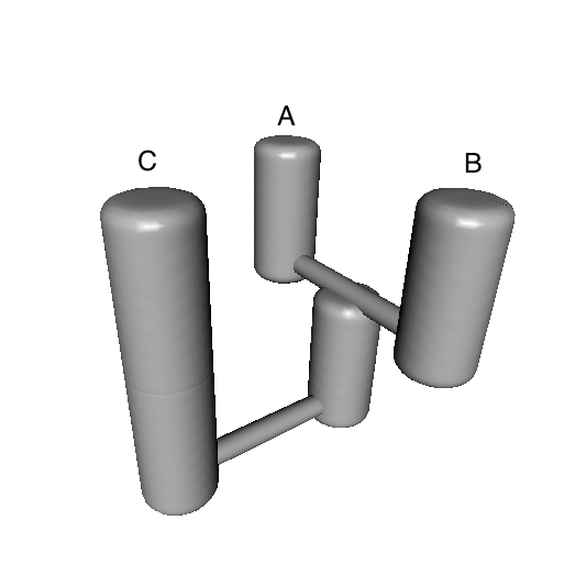
A statuette of this model can then be 3D printed using 14 carat gold, which could be useful as a project souvenir. Just follow this link.
Build your own model
Generating a single* a priori model
What if, instead of or in addition to generating a list of possible models, you would like to create a specific model for which you have some a priori reason to consider alone, or to add to a larger migrationArray as generated above? To do this, you can use the function MakingMigrationIndividualsOneAtATime, whose purpose is to create a single a priori migrationIndividual for a specified coalescence, n0multiplier, growth, and migration history. The four corresponding arguments for this function are collapseList, n0multiplierMapList, growthList and migrationList.
This graphic summary of model objects in PHRAPLwill help you to understand how a model can be modified and customized as much as you want.
collapseList is a list of coalescence history vectors, one vector for each coalescent event in the tree (i.e., for each column in the collapseMatrix. So,
collapseList = list(c(1,1,0),c(2,NA,2))
means that there are two coalescence events: in the first event, populations 1 and 2 coalesce while population 3 does not; in the second event, ancestral population 1-2 coalesces with population 3.
n0multiplierList and growthList are given in the same format as collapseList, and the available parameters for this must match the splitting history depicted in the collapseList. Remember that the n0multiplier parameter is not a parameter for population size, but is rather a population size scalar. So, a model in which population sizes are equal across populations (contemporary and ancestral) would be given as
n0multiplierList = list(c(1,1,1),c(1,NA,1))
If you would like to model one growth rate for tip populations and another growth rate for ancestral populations, this would be given as
growthList = list(c(1,1,1),c(2,NA,2))
Finally, migrationList is a list of migration matrices for the model. There will be one migration matrix for the present generation, plus any historical matrices that apply (there will be as many matrices as there are collapse events). So, in the three population scenario, if there is symmetrical migration between populations 1 and 2 and no historical migration, migrationList will be:
  migrationList<-list(
  t(array(c(
  NA, 1, 0,
  1, NA, 0,
  0, 0, NA),
  dim=c(3,3))),
  t(array(c(
  NA, NA, 0,
  NA, NA, NA,
  0,  NA, NA),
  dim=c(3,3))))
Note that in R, arrays are constructed by reading in values from column 1 first then from column 2, etc. However, it is more intuitive to construct migration matrices by rows (i.e., first listing values for row 1, then row 2, etc.). Thus, here, arrays are typed in by rows and then transposed (using t). Also, spacing and hard returns can be used to visualize these values in the form of matrices.
So, let’s say you want to add one more model to our 48-model migrationArray. Assume that this desired model is the same as model #1 (i.e., migrationArray[[1]], where ((pop1, pop2) pop3))), but where asymmetrical migration rates between sister populations are established at the tips: one rate for pop1 –> pop2 and another rate for pop2 –> pop1. This migrationList would be given as
  migration_1<-t(array(c(
  NA, 1, 0,
  2, NA, 0,
  0, 0, NA),
  dim=c(3,3)))

  migration_2<-t(array(c(
  NA, NA, 0,
  NA, NA, NA,
  0,  NA, NA),
  dim=c(3,3)))
  migrationList<-list(migration_1,migration_2)
So, to produce our desired model, we use the function GenerateMigrationIndividualsOneAtATime:
  migrationIndividual<-GenerateMigrationIndividualsOneAtATime(collapseList=collapseList,
      n0multiplierList=n0multiplierList,growthList=growthList,migrationList=migrationList)
Then, we can add this model to the migrationArray:
  length(migrationArray)
  migrationArray<-c(migrationArray,list(migrationIndividual))
  length(migrationArray)
and view it:
migrationArray[[49]]
Note that a collapseList must always be specified. However, the remaining three parameter matrices are optional, and if they are not specified, null matrices will be automatically produced in which all n0multipliers are set to one, and all growth and migration parameters are set to zero.
Thus, the same migrationIndividual as above can be produced by simply typing
  migrationIndividual<-GenerateMigrationIndividualsOneAtATime(collapseList=collapseList,
      migrationList=migrationList)